Tuning for Concurrency and Performance

Handling Low Latency vs Analytic Jobs

Unlike Spark, SnappyData can distinguish requests that are cheap (low latency) vs requests that require a lot of computational resources (high latency). This is done by a resource scheduler that can balance the needs of many contending users/threads.

For instance, when a SQL client executes a ‘fetch by primary key’ query, there is no need to involve any scheduler or spawn many tasks for such a simple request. The request is immediately delegated to the data node (single thread) and the response is directly sent to the requesting client (probably within a few milliseconds).
In the current version of the product, all query requests that filter on a primary key, a set of keys, or can directly filter using an index are executed without routing to the Job scheduler. Only Row tables can have primary keys or indexes.

When the above conditions are not met, the request is routed to the ‘Lead’ node where the Spark plan is generated and ‘jobs’ are scheduled for execution. The scheduler uses a FAIR scheduling algorithm for higher concurrency, that is, all concurrent jobs are executed in a round-robin manner.

Each job is made up of one or more stages and the planning phase computes the number of parallel tasks for the stage. Tasks from scheduled jobs are then allocated to the logical cores available until all cores are allocated. A round-robin algorithm picks a task from Job1, a task from Job2 and so on. If more cores are available, the second task from Job1 is picked and the cycle continues. But, there are circumstances a single job can completely consume all cores.
For instance, when all cores are available, if a large loading job is scheduled it receives all available cores of which, each of the tasks can be long running. During this time, if other concurrent jobs are assigned, none of the executing tasks is preempted. So, with multiple concurrent users, it is best to avoid running such Jobs using the default high throughput pool.

Computing the Number of Cores for a Job

Executing queries or code in SnappyData results in the creation of one or more Spark jobs. Each Spark job first calculates the number of partitions on the underlying dataset and a task is assigned and scheduled for each partition. But, the number of concurrent tasks executing is limited by the available core count. If the scheduled task count is larger then they will be executed in a staggered manner. Each task is assigned a single core to execute.

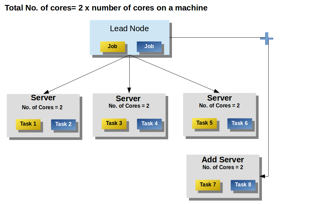
By default, SnappyData sets total available spark executor cores on any data server to be 2 multiplied by the total number of physical cores on a machine.

Spark executor cores = 2 * C
Where C = Total number of physical processor cores on a machine.

This is done keeping in mind some threads which do the IO (Input/Output) reads while the other threads can get scheduled by the operating system. However, increasing this number does not improve query performance.

If you start multiple SnappyData server instances on a machine, then spark.executor.cores should be explicitly set using the following formula:

spark executor cores = N * C
Where N is the number of SnappyData server instaces started on the machine and C = Total number of physical processor cores on a machine.

This can impact thread scheduling and query performance.

Therefore, it is recommended that you maintain only one server per machine so that the total number of threads do not exceed more than twice the number of total physical cores. If you want to run more than one server on a machine, you can use the spark.executor.cores to override the number of cores per server. The cores should be divided accordingly and specified using the spark.executor.cores property.

Spark executor cores = 2 x total physical cores on a machine / No of servers per machine

For example, for a cluster with 2 servers running on two different machines with 4 CPU cores each, a maximum number of tasks that can run concurrently is 16. If a table has 16 partitions (buckets, for the row or column tables), a scan query on this table creates 16 tasks. This means, 16 tasks run concurrently and the last task runs when one of these 16 tasks has finished execution.

SnappyData uses an optimization method which joins multiple partitions on a single machine to form a single partition when there are fewer cores available. This reduces the overhead of scheduling partitions.

In SnappyData, multiple queries can be executed concurrently, if they are submitted by different threads or different jobs. For concurrent queries, SnappyData uses fair scheduling to manage the available resources such that all the queries get a fair distribution of resources.

For example, In the following figure, 6 cores are available on 3 systems, and 2 jobs have 4 tasks each. Because of fair scheduling, both jobs get 3 cores and hence three tasks per job execute concurrently.

Pending tasks have to wait for the completion of the current tasks and are assigned to the core that is first available.

When you add more servers to SnappyData, the processing capacity of the system increases in terms of available cores. Thus, more cores are available so more tasks can concurrently execute.

Configuring the Scheduler Pools for Concurrency

SnappyData out of the box comes configured with two execution pools:

• Low-latency pool: This pool is automatically used when SnappyData determines that a request is of low latency, that is, the queries that are partition pruned to two or fewer partitions.
  

• Default pool: This is the pool that is used for the remaining requests.

Two cores are statically assigned to the low latency pool. Also, the low latency pool has weight twice that of the default pool. Thus, if there are 30 cores available to an executor for a query that has 30 partitions, only 28 would be assigned to it and two cores would be reserved to not starve the low latency queries. When the system has both low latency and normal queries, 20 cores are used for the low latency queries as it has higher priority (weight=2). If a query requires all 30 partitions and no low latency queries are running at that time, all 30 cores are assigned to the first query. However, when a low latency query is assigned, the scheduler does its best to allocate cores as soon as tasks from the earlier query finish.

Applications can explicitly configure to use a particular pool for the current session using a SQL configuration property, snappydata.scheduler.pool. For example, the set snappydata.scheduler.pool=lowlatency command sets the pool as low latency pool for the current session.

New pools can be added and properties of the existing pools can be configured by modifying the conf/fairscheduler.xml file. We do not recommend changing the pool names (default and lowlatency).

Controlling CPU Usage for User Jobs

You can control the CPU usage for user jobs by configuring separate pools for different kinds of jobs.
See configuration here.
The product is configured with two out-of-the-box pools, that is the Default pool and the Low-latency pool. The Default pool has higher priority and also has a minShare, so that some minimum cores are reserved for those jobs if possible. The Stages tab on the SnappyData Monitoring Console shows the available pools. When you track a job for an SQL query on the SQL tab, it shows the pool that is used in the Pool Name column. In-built tasks such as ingestion can show lower priority pools by default to give priority to foreground queries. To configure such priority, do the following:

1. Define the pools in conf/fairscheduler.xml
2. Set a pool for a job using Spark API or use set snappydata.scheduler.pool property in a SnappySession.

To configure the priority based on specific requirements, you can also either permit the users to set the priority for queries or add some pool allocation logic in the application as per client requirements.

Using a Partitioning Strategy to Increase Concurrency

The best way to increasing concurrency is to design your schema such that you minimize the need to run your queries across many partitions. The common strategy is to understand your application patterns and choose a partitioning strategy such that queries often target a specific partition. Such queries will be pruned to a single node and SnappyData automatically optimises such queries to use a single task. For more information see, How to design your schema.

Using Smart Connector for Expanding Capacity of the Cluster

One of the instances, when SnappyData Smart connector mode is useful, is when the computations is separate from the data. This allows you to increase the computational capacity without adding more servers to the SnappyData cluster. Thus, more executors can be provisioned for a Smart Connector application than the number of SnappyData servers.
Also, expensive batch jobs can be run in a separate Smart Connector application and it does not impact the performance of the SnappyData cluster. See, How to Access SnappyData store from an Existing Spark Installation using Smart Connector.

Disabling hashJoin/Aggregate for Cluster Stability

SnappyData has its own operator for extremely fast joins/aggregates. One limitation of this operator is that it stores the objects in Java heap. If heap size is small, it has the potential to cause Garbage Collection (GC) problems and eventually Out-of-memory (OOM). Sometimes, even if the heap size is large this can happen if there are many concurrent queries using these operators. If your use case is such that there will be many joins or aggregates with high cardinality then it is recommended to disable that hashJoin/hashAggregates.

To disable hashJoin/hashAggregates for a particular session you can use the following:

set snappydata.sql.hashAggregateSize=-1
set snappydata.sql.hashJoinSize=-1

To disable hashJoin/hashAggregates for every session, provide the same details in lead.conf file. For example:

-snappydata.sql.hashAggregateSize=-1 -snappydata.sql.hashJoinSize=-1

You must remember that for small dataset the hashJoin operator is much faster than sort merge join. So unless you have a query pattern that can cause high heap usage, it is recommended not to disable hashJoin/hashAggregates.